When we use linear algebra to understand physical systems, we often find more structure in the matrices and vectors than appears in the examples we make up in class. There are many applications of linear algebra; for example, chemists might use row reduction to get a clearer picture of what elements go into a complicated reaction. In this lecture we explore the linear algebra associated with electrical networks.
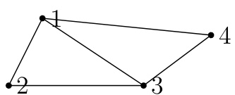
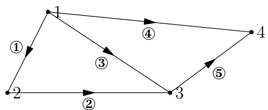
The incidence matrix of this directed graph has one column for each node of the graph and one row for each edge of the graph:
A=−10−1−101−10000110−100011.
If an edge runs from node a to node b , the row corresponding to that edge has −1 in column a and 1 in column b ; all other entries in that row are 0. If we were studying a larger graph we would get a larger matrix but it would be sparse; most of the entries in that matrix would be 0. This is one of the ways matrices arising from applications might have extra structure.
Note that nodes 1, 2 and 3 and edges ①,② and ③ form a loop. The matrix describing just those nodes and edges looks like:
−10−11−10011000.
Note that the third row is the sum of the first two rows; loops in the graph correspond to linearly dependent rows of the matrix.
If the components xi of the vector x describe the electrical potential at the nodes i of the graph, then Ax is a vector describing the difference in potential across each edge of the graph. We see Ax=0 when x1=x2=x3=x4, so the nullspace has dimension 1. In terms of an electrical network, the potential difference is zero on each edge if each node has the same potential. We can’t tell what that potential is by observing the flow of electricity through the network, but if one node of the network is grounded then its potential is zero. From that we can determine the potential of all other nodes of the graph.
The matrix has 4 columns and a 1 dimensional nullspace, so its rank is 3. The first, second and fourth columns are its pivot columns; these edges connect all the nodes of the graph without forming a loop – a graph with no loops is called a tree.
The left nullspace of A consists of the solutions y to the equation: ATy=0 . Since AT has 5 columns and rank 3 we know that the dimension of N(AT) is m−r=2 . Note that 2 is the number of loops in the graph and m is the number of edges. The rank r is n−1 , one less than the number of nodes. This gives us #loops = #edges - (#nodes - 1), or:
number of nodes−number of edges+number of loops=1.
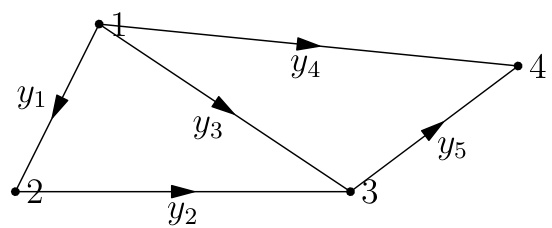
In our example of an electrical network, we started with the potentials xi of the nodes. The matrix A then told us something about potential differences. An engineer could create a matrix C using Ohm’s law and information about the conductance of the edges and use that matrix to determine the current yi on each edge. Kirchhoff’s Current Law then says that ATy=0. , where y is the vector with components y1,y2,y3,y4,y5 . Vectors in the nullspace of AT correspond to collections of currents that satisfy Kirchhoff’s law.
Figure 3: The currents in our graph.
x=x1,x2,x3,x4potentials at nodese=Ax↓x2−x1,etc.potential differencesy=Ce⟶Ohm’s LawATy=0Kirchhoff’s Current Law↑ATyy1,y2,y3,y4,y5currents on edges
Multiplying the first row by the column vector y we get −y1−y3−y4=0 . This tells us that the total current flowing out of node 1 is zero – it’s a balance equation, or a conservation law. Multiplying the second row by y tells us y1−y2=0. ; the current coming into node 2 is balanced with the current going out. Multiplying the bottom rows, we get y2+y3−y5=0 and y4+y5=0 .
We could use the method of elimination on AT to find its column space, but we already know the rank. To get a basis for N(AT) we just need to find two independent vectors in this space. Looking at the equations y1−y2=0 we might guess y1=y2=1 . Then we could use the conservation laws for node 3 to guess y3=−1 and y5=0 . We satisfy the conservation conditions on node 4 with y4=0 , giving us a basis vector 11−100. This vector represents one unit of current flowing around the loop joining nodes 1, 2 and 3; a multiple of this vector represents a different amount of current around the same loop.
We find a second basis vector for N(AT) by looking at the loop formed by nodes 1, 3 and 4: 001−11. The vector 110−11 that represents a current around the outer loop is also in the nullspace, but it is the sum of the first two vectors we found.
We’ve almost completely covered the mathematics of simple circuits. More complex circuits might have batteries in the edges, or current sources between nodes. Adding current sources changes the ATy=0 in Kirchhoff’s current law to ATy=f . Combining the equations e=Ax. , y=Ce and ATy=f gives us:
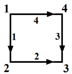
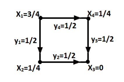
Problem 12.1: (8.2 #1. Introduction to Linear Algebra: Strang) Write down the four by four incidence matrix A for the square graph, shown below. (Hint: the first row has −1 in column 1 and +1 in column 2.) What vectors (x1,x2,x3,x4) are in the nullspace of A? How do you know that (1,0,0,0) is not in the row space of A?
Solution
Solution: The incidence matrix A is written as:
A=−100−11−100011000−11.
To find the vectors in the nullspace, we solve Ax=0 :
so x1=x2=x3=x4 . Therefore, the nullspace consists of vectors of the form (a,a,a,a) .
Finally, (1,0,0,0) is not in the row space of A because it is not orthogonal to the nullspace.
Problem 12.2: (8.2 #7.) Continuing with the network from problem one, suppose the conductance matrix is
C=1000020000200001.
Multiply matrices to find ATCA . For f=(1,0,−1,0), , find a solution to ATCA˙x=f. Write the potentials x and currents y=−CAx on the square graph (see above) for this current source f going into node 1 and out from node 3.
Solution
Solution: From the previous question, we know that the incidence matrix is: